Two Level Quantization Formats (MX4, MX6, MX9: shared Microexponents)#
Note
In this documentation, AMD Quark is sometimes referred to simply as “Quark” for ease of reference. When you encounter the term “Quark” without the “AMD” prefix, it specifically refers to the AMD Quark quantizer unless otherwise stated. Please do not confuse it with other products or technologies that share the name “Quark.”
AMD Quark supports the MX6 and MX9 quantization formats through quark.torch, as introduced in With Shared Microexponents, A Little Shifting Goes a Long Way.
The novelty of these quantization formats lies in the way quantization scales are computed and stored. For a general introduction to quantization and its use in AMD Quark, refer to the Quantization with AMD Quark documentation.
Context: Uniform Integer Quantization#
Quantization typically aims to use fewer bits per weight of a high-precision matrix \(W\) of shape \([m, n]\), originally in float32, float16, or bfloat16 precision. A classic quantization technique is uniform integer quantization, such as INT8 quantization, which uses the following scheme:
Here, \(s\) is the scale factor, \(x_Q\) represents a quantized value (e.g., an int8 value), and \(x_R\) represents the high-precision value (typically float16, bfloat16, or float32).
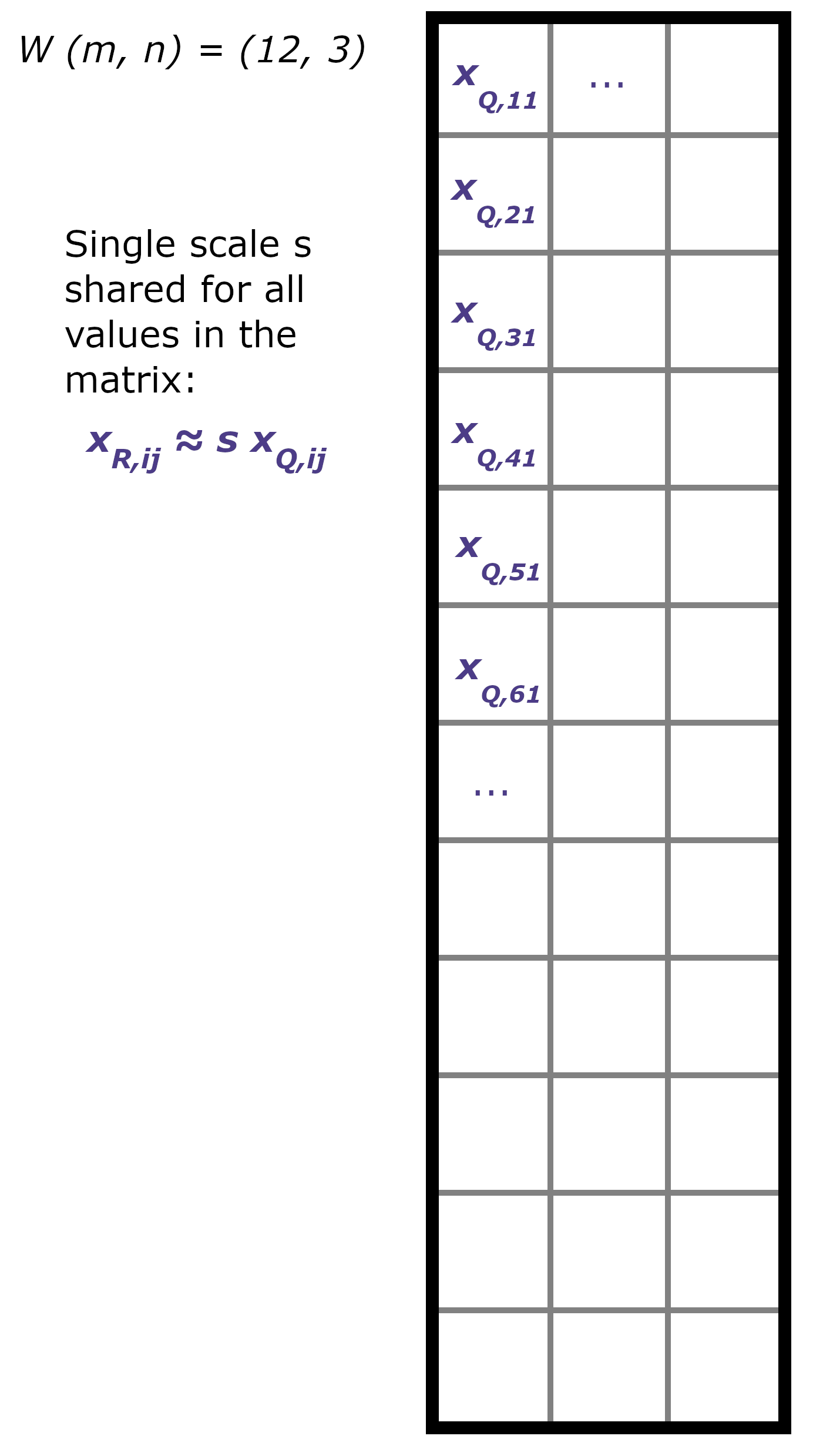
Uniform integer per-tensor quantization.#
Such a quantization scheme necessarily leads to quantization error. To preserve model prediction quality, a strategy is to allow more granular scales. For example, instead of computing a single scale \(s\) for the whole matrix \(W\), increase the granularity by computing one scale per column, or even one scale per group of size \(k\) within a column, as shown below.
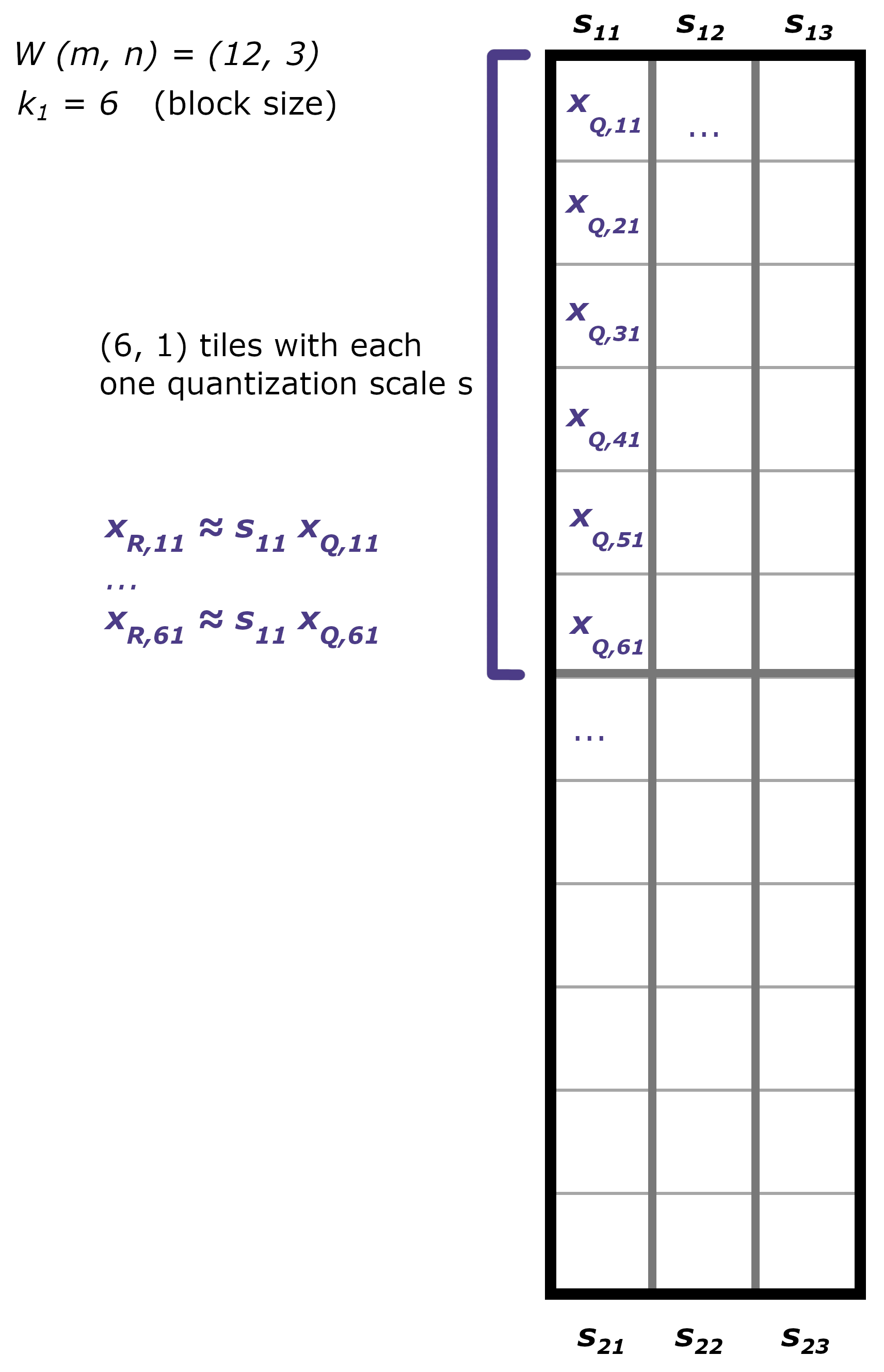
Per-block quantization, with the block size \(k_1 = 6\).#
Increasing this granularity effectively means considering only a subset of values from \(W\) to compute the relevant scale \(s\) for this subset.
Another strategy to balance quantization error with the number of bits per weight is to use a different data type to store the scales. A common approach is to store scales as float16 or float32 values, but scales can also be constrained to be powers of two, implementing the dequantization operation \(s \times x_Q\) as a simple bit shift (similarly for the quantization operation). Thus, instead of storing the scale \(s\) on 16 or 32 bits, it can be stored on a lower bitwidth, e.g., 8 bits.
Two-level Quantization: MX6 and MX9 Data Types#
Refer to MX9, MX6, and MX4 specifications from [1]. The MX6 and MX9 data types leverage both the granularity of the scale factors and the precision allocated to them to:
Minimize the number of bits per weight
Minimize degradation in predictive performance due to quantization
Be hardware-friendly
To achieve these goals, the classic quantization scheme \(x_R = s \times x_Q\) is decomposed into
x_R = s_b \times s_{sb} \times x_Q
where \(s_b\) stands for the block scale (1st level), and \(s_{sb}\) stands for the subblock scale (2nd level).
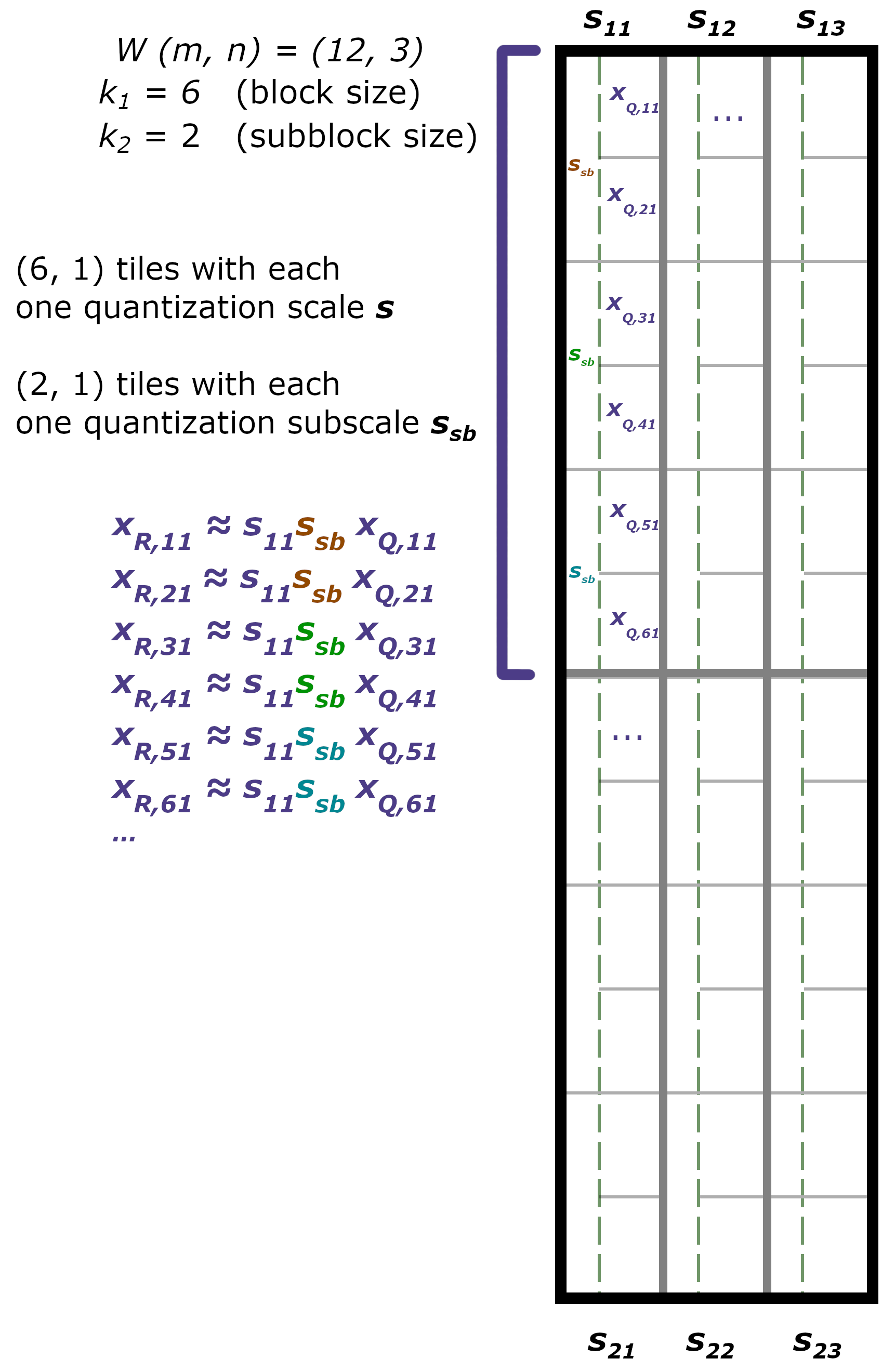
A dummy example for a two-level quantization scheme, with the block size \(k_1 = 6\). The different colors for \(s_{sb}\) indicate different values per subblock.#
For example, in the MX9 data type, the block scale \(s_b\) is an 8-bit (\(d_1 = 8\)) power of two (within \([2^{-127}, ..., 2^{127}]\)) scale, shared over \(k_1 = 16\) values, while the subblock scale \(s_{sb}\) is a 1-bit (\(d_2 = 1\)) power of two scale (effectively, \(2^{0}\) or \(2^{-1}\)) shared over \(k_2 = 2\) values.
The mantissa bit-width \(m\) represents the number of bits used to store the quantized value \(x_Q\), effectively using \(2^m\) possible different bins.
The total number of bits per value is
(m + 1) + \frac{d_1}{k_1} + \frac{d_2}{k_2}
where \(m + 1\) accounts for the sign bit and the \(m\) bits for storing \(x_Q\), and the two other terms split the storing cost of \(s_b\) and \(s_{sb}\) over the values within the block and subblock.
The intuition behind this quantization scheme is that while a few block scales \(s_b\) are stored in relatively high precision (8 bits per scale per block of 16 values), many more subscales \(s_{sb}\) are stored (with \(k_2 = 2\), half the number of values in the matrix) to allow for lower quantization error for each floating point value in subblocks. As these subscales use a very low bitwidth (1 bit), it is a storage (and compute, as bit shifts are used) cost that can be afforded.
How are These Two-Level Scales Obtained?#
Several strategies can be chosen, as long as they respect the constraints on the scales and sub-scales. In AMD Quark, this can be found at quark/torch/kernel/hw_emulation/hw_emulation_interface.py. The scales and sub-scales are computed as follows (using MX9 as an example):
From the original float32, bfloat16, or float16 \(W\) matrix, retrieve the maximum power of two exponent of each block of size \(k_1 = 16\), denoted \(e_{b,max}\). This can be retrieved from the exponent bits from the floating point representation \((-1)^s2^e \times 1.m\).
For each subblock of \(k_2 = 2\) values within the block, determine whether both floating point values have an exponent strictly smaller than \(e_{b,max}\).
If that is the case, the values within the block are comparatively small, hence a smaller scale is desired, which amounts to a smaller quantization range and finer quantization of small values. Choose \(s_{sb} = 2^{-1}\).
If that is not the case, choose \(s_{sb} = 1\) (no bit shift, no subscale really applied).
The block scale is chosen as \(s_b = 2^{e_{b,max} - 8 + 2}\), where the \(2^{-(8 - 1 - 1)}\) term is an implementation detail accounting for the hidden bit of floating point numbers, and base 2 to base 10 conversion of the mantissa \((1.m)_2\) [1].
Finally, the global scale for a subblock of two values is \(s = s_b \times s_{sb} = 2^{e_{b,max} - 8 + 2} \times 2^{(\text{-1 or 0})}\).
Hardware Mapping#
Why is this quantization scheme interesting in terms of mapping it to hardware?
One element is that scaling can be implemented as bit shifts, both for the block scales and subblock scales, as these are stored as powers of two.